うさぎでもわかる微分方程式 Part15 ラプラス変換を用いた微分方程式・連立微分方程式の解き方
こんにちは、ももやまです。
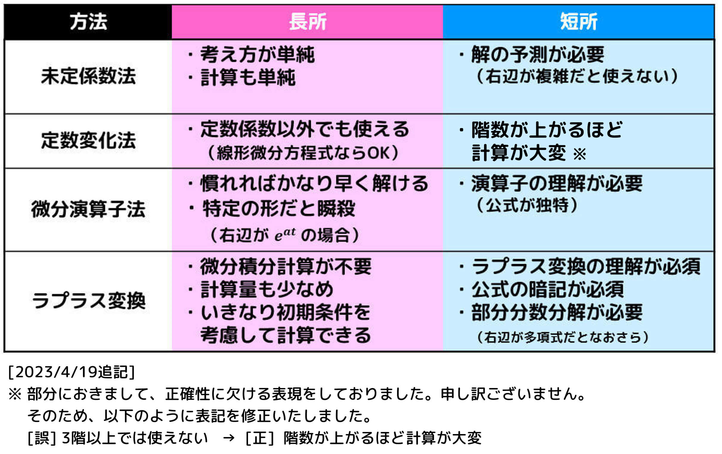
今回は、非同次の定数係数線形微分方程式の4つの解き方
の中の最後の1つである「ラプラス変換を用いた微分方程式の解き方」について説明します。
残りの3つの特殊解を求める方法の長所・短所も載せておくので、特殊解をどう求めようか迷った人はご覧ください。

なお、ラプラス変換の基礎についての詳しい記事は、こちらをご覧ください。
目次
1.覚えるべきラプラス変換の法則・公式
まずは、ラプラス変換で頭にいれておくべき法則・公式を確認しておきましょう。
(1) 重要法則

(2) 重要公式

移動の法則を適用した形
- \( e^{at} t^n \)
- \( e^{at} \sin bt \)
- \( e^{at} \cos bt \)
の3つのラプラス変換を覚え、必要に応じて \( n = 0 \), \( a = 0 \) などを代入してから
- \( t^n \)
- \( e^{at} \)
- \( \sin bt \)
- \( \cos bt \)
などのラプラス変換を導出するのが私のおすすめです。
(覚える公式を少なくできるため)
(3) ラプラス変換表
実際にラプラス変換を求めて微分方程式を求める際には、下のようなラプラス変換表からある関数 \( f(t) \) と、ラプラス変換後の関数 \( F(s) \) の対応が読み解ければOKです。
| 時間関数 \( f(t) \) | ラプラス変換 \( F(s) \) | 時間関数 \( f(t) \) | ラプラス変換 \( F(s) \) |
|---|---|---|---|
| \( 1 \) | \[ \frac{1}{s} \] | \( e^{ \textcolor{red}{a} t} \) | \[ \frac{1}{s- \textcolor{red}{a} } \] |
| \( t^{\textcolor{purple}{n}} \) | \[ \frac{ \textcolor{purple}{n} !}{s^{ \textcolor{ purple }{n} +1}} \] | \( e^{ \textcolor{red}{a} t} t^{\textcolor{ purple }{n} }\) | \[ \frac{ \textcolor{ purple }{n} ! }{ (s- \textcolor{red}{a} )^{ \textcolor{ purple }{n} + 1 } } \] |
| \( \sin \textcolor{blue}{b} t \) | \[ \frac{ \textcolor{blue}{b} }{s^2 + \textcolor{blue}{b}^2 } \] | \( e^{ \textcolor{red}{a} t} \sin \textcolor{blue}{b} t \) | \[ \frac{ \textcolor{blue}{b} }{ (s- \textcolor{red}{a} )^2 + \textcolor{blue}{b}^2 } \] |
| \( \cos \textcolor{blue}{b} t \) | \[ \frac{ s }{s^2 + \textcolor{blue}{b}^2 } \] | \( e^{ \textcolor{red}{a} t} \cos \textcolor{blue}{b} t \) | \[ \frac{ s - \textcolor{red}{a} }{ (s- \textcolor{red}{a} )^2 + \textcolor{blue}{b}^2 } \] |
(i) ラプラス変換をする場合
ラプラス変換は、表の左側 \( f(t) \) から右側 \( F(s) \) への変換に相当します。
例えば、\( f(t) = t^{\textcolor{purple}{2}} \) をラプラス変換すると考えましょう。まず、左側に \( t^2 \) に該当する項目がないかを探します。
すると、\( f(t) = t^{\textcolor{purple}{n}} \) の \( \textcolor{purple}{n = 2} \) のときが該当しますね。該当する項目( \( t^{\textcolor{purple}{n}} \) の右側を見ると、\[
\frac{ \textcolor{purple}{n} !}{s^{ \textcolor{purple}{n} +1}}
\]と書かれていますね。ここに \( \textcolor{purple}{n = 2} \) を入れた\[
\frac{2!}{s^{3}}
\]が \( t^2 \) のラプラス変換の結果に相当します。
(ii) ラプラス逆変換をする場合
ラプラス逆変換は、表の右側 \( F(s) \) から左側 \( f(t) \) への変換に相当します。
例えば、\[ \frac{1}{s-\textcolor{red}{5}} \] をラプラス変換すると考えましょう。まず、右側に \( \frac{1}{s- \textcolor{red}{5} } \) に該当する項目がないかを探します。
すると、\[ F(s) = \frac{1}{s- \textcolor{red}{a} } \] の \( \textcolor{red}{a=5} \) のときが該当しますね。該当する項目( \( \frac{1}{s- \textcolor{red}{5} } \) の左側を見ると、\( e^{ \textcolor{red}{a} t} \) と書かれていますね。ここに \( \textcolor{red}{a=5} \) を入れた\[
e^{ \textcolor{red}{5} t}
\]が \( \frac{1}{s- \textcolor{red}{5} } \) のラプラス逆変換の結果に相当します。
(iii) PDF版ラプラス変換表
上のボタンからラプラス変換表をダウンロードを行うことができます!
計算の際などに是非ご利用ください。
2.ラプラス変換を用いた微分方程式の解き方
では、さっそくラプラス変換を用いた微分方程式の解き方を例題を踏まえて説明していきましょう。
(なお、ラプラス変換の表記に合わせて \( t \) の微分に関する微分方程式にしています。)
例題1
微分方程式\[
\frac{d^2y}{dt^2} - 4 \frac{dy}{dt} + 3y = e^{2t}
\]を初期条件 \( y(0) = 0 \), \( y'(0) = 0 \) の下で解きなさい。
解説1
ラプラス変換を用いた微分方程式は4ステップで解くことができます。
Step1. 微分方程式を立てる(ほとんどの場合必要なし)
力学などの物理科目の場合の場合、微分方程式を立てるところから始まります。
ただし、数学科目の場合、あらかじめ問題文に式が与えられていることがほとんどなのでこのステップは必要ありません。
Step2. 両辺をラプラス変換し、F(s)に関する方程式へ
次に、微分方程式の解を \( y = f(t) \) をおき、両辺をラプラス変換します*1。
(つまり \( \color{magenta}{f(0)} = 0 \), \( \color{orange}{f'(0)} = 0 \))
ここで、\[\begin{align*}
\mathcal{L} \left[ \frac{d^2y}{dt^2} \right] & = \mathcal{L} \left[ f''(t) \right]
\\ & = s^2 F(s) - s \color{magenta}{f(0)} - \color{orange}{f'(0)}
\\ & = s^2 F(s)
\end{align*}\]
\[\begin{align*}
\mathcal{L} \left[ \frac{dy}{dt} \right] & = \mathcal{L} \left[ f'(t) \right]
\\ & = s F(s) - \color{magenta}{f(0)}
\\ & = s F(s)
\end{align*}\]
\[\begin{align*}
\mathcal{L} \left[ e^{\color{red}{2}t} \right] & = \frac{1}{ s - \color{red}{2} }
\end{align*}\]
なので、両辺をラプラス変換すると、\[\begin{align*}
\mathcal{L} \left[ \frac{d^2y}{dt^2} - 4 \frac{dy}{dt} + 3y \right] & = \mathcal{L} \left[ e^{2t} \right] \\
\mathcal{L} \left[ f''(t) \right] - 4 \mathcal{L} \left[ f'(t) \right] + 3 \mathcal{L} \left[ f(t) \right] & = \mathcal{L} \left[ e^{2t} \right] \\
s^2 F(s) - 4sF(s) + 3F(s) & = \frac{1}{s-2}
\end{align*}\]となります。
ラプラス変換を用いることで、もとの微分方程式\[
\frac{d^2y}{dt^2} - 4 \frac{dy}{dt} + 3y = e^{2t} \\
y(0) = 0, \ \ \ y'(0) = 0
\]を\[
s^2 F(s) - 4sF(s) + 3F(s) = \frac{1}{s-2}
\]のようなただの方程式に変換することができるのです!
微分方程式を求めるためには微積分が必要ですが、ただの方程式であれば微積分なしに解くことができます!
Step3. F(s)を求める
つぎに、(2)で出てきた \( F(s) \) の方程式から、\( F(s) \) を求めます。
(2)の式は、\[\begin{align*}
s^2 F(s) - 4sF(s) + 3F(s) & = \frac{1}{s-2} \\
(s^2 - 4s + 3)F(s) & = \frac{1}{s-2} \\
(s-1)(s-3) F(s) & = \frac{1}{s-2}
\end{align*}\]と変形することで、\[
F(s) = \frac{1}{(s-1)(s-2)(s-3)}
\]と求めることができます。
Step4. あとはラプラス逆変換するだけ!
方程式が求められても、最後にラプラス逆変換を行うことで、元の形 \( f(t) \) に戻してあげる必要があります。
ここの計算で、部分分数分解を使うので場合によっては大変かもしれません。
\( F(s) \) を部分分数分解すると、\[\begin{align*}
F(s) & = \frac{1}{(s-1)(s-2)(s-3)}
\\ & = \frac{1}{2} \frac{1}{s-1} - \frac{1}{s-2} + \frac{1}{2} \frac{1}{s-3}
\end{align*}\]となるので、\[\begin{align*}
f(t) & = \mathcal{L}^{-1} \left[ F(s) \right]
\\ & = \mathcal{L}^{-1} \left[ \frac{1}{(s-1)(s-2)(s-3)} \right]
\\ & = \frac{1}{2} \mathcal{L}^{-1} \left[ \frac{1}{s - \textcolor{red}{1}} \right] - \mathcal{L}^{-1} \left[ \frac{1}{s - \textcolor{red}{2}} \right] + \frac{1}{2} \mathcal{L}^{-1} \left[ \frac{1}{s - \textcolor{red}{3}} \right]
\\ & = \frac{1}{2} e^{ \textcolor{red}{1} t } - e^{ \textcolor{red}{2} t } + \frac{1}{2} e^{ \textcolor{red}{3} t }
\\ & = \frac{1}{2} e^t - e^{2t} + \frac{1}{2} e^{3t}
\end{align*}\]と求めることができる。
よって、微分方程式の解は\[
y = \frac{1}{2} e^t - e^{2t} + \frac{1}{2} e^{3t}
\]となる。
このように、
- 微分方程式を立てる
- 微分方程式をラプラス変換し、\( F(s) \) に関する方程式へ
- \( F(s) \) を求める
- \( F(s) \) をラプラス逆変換し、\( y = f(t) \) に関する式へ
ように、途中でラプラス変換・ラプラス逆変換を挟むことで微積分の必要がなく、簡単な代数計算だけで微分方程式を求めることができるのです!

3.ラプラス変換を用いた連立微分方程式の解き方
ラプラス変換を用いることで、連立微分方程式も解くことができます。
実際に例題で解き方の流れを確認していきましょう。
例題2
連立微分方程式\[
\left\{ \begin{array}{l} \frac{dx}{dt} = x + 2y + e^{2t} \\ \frac{dy}{dt} = 2x + y + 2e^{2t} \end{array}\right.
\]を初期条件 \( x(0) = 0 \), \( y(0) = 0 \) の下で解きなさい。
解説2
Step1. 連立微分方程式の立式
今回のように、あらかじめ解くべき問題が用意されている場合は不要です。
Step2. ラプラス変換を行い連立方程式に変形
関数 \( x(t) \), \( y(t) \) のラプラス変換をそれぞれ \( X(s) \), \( Y(s) \) とおきます。
ここで、\( \textcolor{magenta}{x(0)} = 0 \), \( \textcolor{orange}{y(0)} = 0 \) なので*2、
\[\begin{align*}
\mathcal{L} \left[ \frac{dx}{dt} \right] & = \mathcal{L} \left[ x'(t) \right]
\\ & = s X(s) - \textcolor{magenta}{x(0)}
\\ & = s X(s)
\end{align*}\]
\[\begin{align*}
\mathcal{L} \left[ \frac{dy}{dt} \right] & = \mathcal{L} \left[ y'(t) \right]
\\ & = s Y(s) - \textcolor{orange}{y(0)}
\\ & = s Y(s)
\end{align*}\]となります。
よって、それぞれの微分方程式\[
\left\{ \begin{array}{l} \frac{dx}{dt} = x + 2y + e^{2t} \\ \frac{dy}{dt} = 2x + y + 2e^{2t} \end{array}\right.
\]を両辺でラプラス変換すると、\[
\left\{ \begin{array}{l} s X(s) = X(s) + 2Y(s) + \frac{1}{s-2} \\ s Y(s) = 2X(s) + Y(s) + \frac{2}{s-2} \end{array}\right. \]\[
\left\{ \begin{array}{l} (s-1) X(s) - 2Y(s) =\frac{1}{s-2} \\ -2X(s) + (s-1) Y(s) = \frac{2}{s-2} \end{array}\right.
\]となり、ただの連立方程式になりますね。
連立微分方程式であれば解くのは大変かもしれませんが、ただの連立方程式であれば微分積分なしに解くことができますね!
Step3. 連立方程式を解く
ここからは線形代数の力を使って連立微分方程式を解きます。
逆行列の求め方や、逆行列を用いた連立方程式の解き方を忘れてしまった人はこちらから復習しましょう。
ここで、先程の連立方程式を行列を用いて表すと、\[
\left( \begin{array}{ccc} (s-1) X(s) - 2Y(s) = \frac{1}{s-2} \\ -2X(s) + (s-1) Y(s) = \frac{2}{s-2} \end{array} \right) \\
\left( \begin{array}{ccc} s-1 & -2 \\ -2 & s-1 \end{array} \right) \left( \begin{array}{ccc} X(s) \\ Y(s) \end{array} \right) = \left( \begin{array}{ccc} \frac{1}{s-2} \\ \frac{2}{s-2} \end{array} \right)
\]と、\( A \vec{x} = \vec{b} \) の形に変形できますね。
ここで、\[\begin{align*}
|A| & = \left| \begin{array}{ccc} s-1 & -2 \\ -2 & s-1 \end{array} \right| \\ & = (s-1)^2 + 4
\\ & = s^2 -2s - 3
\\ & = (s-3)(s+1) \not = 0
\end{align*}\]なので、行列 \( A \) に逆行列*3が存在しますね。
そのため、連立方程式を\[\begin{align*}
\left( \begin{array}{ccc} X(s) \\ Y(s) \end{array} \right) & = \left( \begin{array}{ccc} s-1 & -2 \\ -2 & s-1 \end{array} \right)^{-1} \left( \begin{array}{ccc} \frac{1}{s-2} \\ \frac{2}{s-2} \end{array} \right)
\\ & = \frac{1}{(s-3)(s+1)} \left( \begin{array}{ccc} s-1 & 2 \\ 2 & s-1 \end{array} \right) \left( \begin{array}{ccc} \frac{1}{s-2} \\ \frac{2}{s-2} \end{array} \right)
\\ & = \frac{1}{(s-3)(s+1)} \left( \begin{array}{ccc} s-1 & 2 \\ 2 & s-1 \end{array} \right) \left( \begin{array}{ccc} \frac{1}{s-2} \\ \frac{2}{s-2} \end{array} \right)
\\ & = \frac{1}{(s-3)(s+1)(s-2)} \left( \begin{array}{ccc} s+3 \\ 2s \end{array} \right)
\end{align*}\]と計算することができます*4。
よって、\( X(s) \), \( Y(s) \) の解は\[
\left\{ \begin{array}{l} X(s) = \frac{s+3}{(s-3)(s+1)(s-2)} \\ Y(s) = \frac{2s}{(s-3)(s+1)(s-2)} \end{array}\right.
\]と求めることができます。
Step4. あとはラプラス逆変換するだけ!
最後に \( X(s) \), \( Y(s) \) それぞれでラプラス逆変換を行い、\( x(t) \), \( y(t) \) を求める必要があります。
ここでも部分分数分解を使うことが多いので、部分分数分解が苦手な人にはちょっと大変かもしれません。
\( X(s) \), \( Y(s) \) を部分分数分解すると、\[\begin{align*}
X(s) & = \frac{s+3}{(s-3)(s+1)(s-2)}
\\ & = \frac{3}{2} \frac{1}{s-3} + \frac{1}{6} \frac{1}{s+1} - \frac{5}{3} \frac{1}{s-2}
\end{align*}\]\[\begin{align*}
Y(s) & = \frac{2s}{(s-3)(s+1)(s-2)}
\\ & = \frac{3}{2} \frac{1}{s-3} - \frac{1}{6} \frac{1}{s+1} - \frac{4}{3} \frac{1}{s-2}
\end{align*}\]となります。
よって、ラプラス逆変換を行うことで \( x(t) \), \( y(t) \) を\[\begin{align*}
x(t) & = \mathcal{L}^{-1} \left[ X(s) \right]
\\ & = \mathcal{L}^{-1} \left[ \frac{s+3}{(s-3)(s+1)(s-2)} \right]
\\ & = \frac{3}{2} \mathcal{L}^{-1} \left[ \frac{1}{s-\textcolor{red}{3}} \right] + \frac{1}{6} \mathcal{L}^{-1} \left[ \frac{1}{s- (\textcolor{red}{-1})} \right] - \frac{5}{3} \mathcal{L}^{-1} \left[ \frac{1}{s-\textcolor{red}{2}} \right]
\\ & = \frac{3}{2} e^{\textcolor{red}{3} t} + \frac{1}{6} e^{\textcolor{red}{-1} t} - \frac{5}{3} e^{\textcolor{red}{2} t}
\\ & = \frac{3}{2} e^{3t} + \frac{1}{6} e^{-t} - \frac{5}{3} e^{2t}
\end{align*}\]
\[\begin{align*}
y(t) & = \mathcal{L}^{-1} \left[ Y(s) \right]
\\ & = \mathcal{L}^{-1} \left[ \frac{2s}{(s-3)(s+1)(s-2)} \right]
\\ & = \frac{3}{2} \mathcal{L}^{-1} \left[ \frac{1}{s-\textcolor{red}{3}} \right] - \frac{1}{6} \mathcal{L}^{-1} \left[ \frac{1}{s- (\textcolor{red}{-1})} \right] - \frac{4}{3} \mathcal{L}^{-1} \left[ \frac{1}{s-\textcolor{red}{2}} \right]
\\ & = \frac{3}{2} e^{\textcolor{red}{3} t} - \frac{1}{6} e^{\textcolor{red}{-1} t} - \frac{4}{3} e^{\textcolor{red}{2} t}
\\ & = \frac{3}{2} e^{3t} - \frac{1}{6} e^{-t} - \frac{4}{3} e^{2t}
\end{align*}\]
と求めることができます。
よって、微分方程式の解は\[
\left\{ \begin{array}{l} x = \frac{3}{2} e^{3t} + \frac{1}{6} e^{-t} - \frac{5}{3} e^{2t} \\ y= \frac{3}{2} e^{3t} - \frac{1}{6} e^{-t} - \frac{4}{3} e^{2t} \end{array}\right.
\]となります。
このように、
- 連立微分方程式を立てる
- 連立微分方程式をラプラス変換し、\( X(s) \), \( Y(s) \) に関する連立方程式へ
- 連立微分方程式を解き、\( X(s) \), \( Y(s) \) を求める
- \( X(s) \), \( Y(s) \) をラプラス逆変換し、\( x(t) \), \( y(t) \) に戻す
ことで、途中でラプラス変換・ラプラス逆変換を挟むことで微積分をせずに代数計算だけで連立微分方程式も求めることができるのです!

4.練習問題
では、5問ほど練習をしてみましょう。
練習1
微分方程式\[
\frac{d^2y}{dt^2} - 3 \frac{dy}{dt} +2y = e^{t}
\]を初期条件 \( y(0) = 1 \), \( y'(0) = 1 \) の下で解きなさい。
練習2
微分方程式\[
\frac{d^2y}{dt^2} - 4 \frac{dy}{dt} + 4y = \sin 2t
\]を初期条件 \( y(0) = 0 \), \( y'(0) = 0 \) の下で解きなさい。
練習3
微分方程式\[
\frac{d^2y}{dt^2} - 2 \frac{dy}{dt} + 2y = 2t
\]を初期条件 \( y(0) = 0 \), \( y'(0) = 0 \) の下で解きなさい。
練習4
つぎの連立微分方程式\[
\left\{ \begin{array}{l} \frac{dx}{dt} + 2y = 2 e^{t} \\ 2x + \frac{dy}{dt} = e^t \end{array}\right.
\]の解を初期条件 \( x(0) = 0 \), \( y(0) = 0 \) に基づいて解きなさい。
5.練習問題の答え
解答1
解を \( y = f(t) \) をおき、両辺をラプラス変換する。
すると、\( \textcolor{magenta}{f(0)} = 1 \), \( \textcolor{orange}{f'(0)} = 1 \) となる。
ここで、\[\begin{align*}
\mathcal{L} \left[ \frac{d^2y}{dt^2} \right] & = \mathcal{L} \left[ f''(t) \right]
\\ & = s^2 F(s) - s \textcolor{magenta}{f(0)} - \textcolor{orange}{f'(0)}
\\ & = s^2 F(s) - s - 1
\end{align*}\]
\[\begin{align*}
\mathcal{L} \left[ \frac{dy}{dt} \right] & = \mathcal{L} \left[ f'(t) \right]
\\ & = s F(s) - \textcolor{magenta}{f(0)}
\\ & = s F(s) - 1
\end{align*}\]
なので、両辺をラプラス変換すると、\[\begin{align*}
\mathcal{L} \left[ \frac{d^2y}{dt^2} - 3 \frac{dy}{dt} + 2y \right] & = \mathcal{L} \left[ e^{t} \right] \\
\mathcal{L} \left[ f''(t) \right] - 3 \mathcal{L} \left[ f'(t) \right] + 2 \mathcal{L} \left[ f(t) \right] & = \mathcal{L} \left[ e^{\textcolor{red}{1}t} \right] \\
s^2 F(s) - s - 1 - 3 (sF(s) - 1) + 2F(s) & = \frac{1}{s-\textcolor{red}{1}} \\
s^2 F(s) - 3s F(s) + 2 F(s) & = \frac{1}{s-1} + s - 2
\end{align*}\]となる。
よって、\( F(s) \) を\[\begin{align*}
s^2 F(s) - 3sF(s) + 2F(s) & = \frac{1}{s-1} + s - 2 \\
(s^2 - 3s + 2)F(s) & = \frac{(s-2)(s-1)+1}{s-1} \\
(s-1)(s-2) F(s) & = \frac{s^2-3s+3}{s-1}
\end{align*}\]と変形することで、\[
F(s) = \frac{s^2-3s+3}{(s-1)^2(s-2)}
\]と求めることができる。
ここで、\( F(s) \) を部分分数分解すると、\[\begin{align*}
F(s) & = \frac{s^2-3s+3}{(s-1)^2(s-2)}
\\ & = \frac{1}{s-2} - \frac{1}{(s-1)^2}
\end{align*}\]となるので、\[\begin{align*}
f(t) & = \mathcal{L}^{-1} \left[ F(s) \right]
\\ & = \mathcal{L}^{-1} \left[ \frac{s^2-3s+3}{(s-1)^2(s-2)} \right]
\\ & = \mathcal{L}^{-1} \left[ \frac{1}{s - \textcolor{red}{2}} \right] - \mathcal{L}^{-1} \left[ \frac{\textcolor{blue}{1}!}{(s - \textcolor{red}{1})^{\textcolor{blue}{1} + 1} } \right]
\\ & = e^{ \textcolor{red}{2} t } - t^{ \textcolor{blue}{1} } e^{ \textcolor{red}{1} t }
\\ & = e^{2t} - t e^{t}
\end{align*}\]と求めることができる。
よって、微分方程式の解は\[
y = e^{2t} - t e^{t}
\]となる。
解答2
解を \( y = f(t) \) をおき、両辺をラプラス変換する。
すると、\( \textcolor{magenta}{f(0)} = 0 \), \( \textcolor{orange}{f'(0)} = 0 \) となる。
ここで、\[\begin{align*}
\mathcal{L} \left[ \frac{d^2y}{dt^2} \right] & = \mathcal{L} \left[ f''(t) \right]
\\ & = s^2 F(s) - s \textcolor{magenta}{f(0)} - \textcolor{orange}{f'(0)}
\\ & = s^2 F(s)
\end{align*}\]
\[\begin{align*}
\mathcal{L} \left[ \frac{dy}{dt} \right] & = \mathcal{L} \left[ f'(t) \right]
\\ & = s F(s) - \textcolor{magenta}{f(0)}
\\ & = s F(s)
\end{align*}\]
なので、両辺をラプラス変換すると、\[\begin{align*}
\mathcal{L} \left[ \frac{d^2y}{dt^2} - 4 \frac{dy}{dt} + 4y \right] & = \mathcal{L} \left[ \sin \textcolor{blue}{2} t \right] \\
\mathcal{L} \left[ f''(t) \right] - 4 \mathcal{L} \left[ f'(t) \right] + 4 \mathcal{L} \left[ f(t) \right] & = \mathcal{L} \left[ \sin \textcolor{blue}{2} t \right] \\
s^2 F(s) - 4s F(s) + 4 F(s) & = \frac{ \textcolor{blue}{2} }{ s^2 + \textcolor{blue}{2}^2 } \\
s^2 F(s) - 4s F(s) + 4 F(s) & = \frac{2}{s^2 + 4}
\end{align*}\]となる。
よって、\( F(s) \) を\[\begin{align*}
s^2 F(s) - 4s F(s) + 4 F(s) & = \frac{2}{s^2 + 4} \\
(s - 2)^2 F(s) & = \frac{2}{s^2 + 4}
\end{align*}\]と変形することで、\[
F(s) = \frac{2}{(s-2)^2 (s^2 + 4)}
\]と求めることができる。
ここで、\( F(s) \) を部分分数分解すると、\[\begin{align*}
F(s) & = \frac{2}{(s-2)^2 (s^2 + 4)}
\\ & = \frac{1}{8} \frac{s}{s^2+4} - \frac{1}{8} \frac{1}{s-2} + \frac{1}{4} \frac{1}{(s-2)^2}
\end{align*}\]となるので、\[\begin{align*}
f(t) & = \mathcal{L}^{-1} \left[ F(s) \right]
\\ & = \mathcal{L}^{-1} \left[ \frac{2}{(s-2)^2 (s^2 + 4)} \right]
\\ & = \frac{1}{8} \mathcal{L}^{-1} \left[ \frac{s}{s^2+\textcolor{blue}{2}^2} \right] - \frac{1}{8} \mathcal{L}^{-1} \left[ \frac{1}{ s - \textcolor{red}{2} } \right] + \frac{1}{4} \mathcal{L}^{-1} \left[ \frac{\textcolor{blue}{1}!}{(s - \textcolor{red}{2})^{\color{blue}{1} + 1} } \right]
\\ & = \frac{1}{8} \cos \textcolor{blue}{2} t - \frac{1}{8} e^{ \textcolor{red}{2} t } + \frac{1}{4} t^{ \textcolor{blue}{1} } e^{ \textcolor{red}{2} t }
\\ & = \frac{1}{8} \cos 2t - \frac{1}{8} e^{2t} + \frac{1}{4} t e^{2t}
\end{align*}\]と求めることができる。
よって、微分方程式の解は\[
y = \frac{1}{8} \cos 2t - \frac{1}{8} e^{2t} + \frac{1}{4} t e^{2t}
\]となる。
解答3
解を \( y = f(t) \) をおき、両辺をラプラス変換する。
すると、\( \textcolor{magenta}{f(0)} = 0 \), \( \textcolor{orange}{f'(0)} = 1 \) となる。
ここで、\[\begin{align*}
\mathcal{L} \left[ \frac{d^2y}{dt^2} \right] & = \mathcal{L} \left[ f''(t) \right]
\\ & = s^2 F(s) - s \textcolor{magenta}{f(0)} - \textcolor{orange}{f'(0)}
\\ & = s^2 F(s) - 1
\end{align*}\]
\[\begin{align*}
\mathcal{L} \left[ \frac{dy}{dt} \right] & = \mathcal{L} \left[ f'(t) \right]
\\ & = s F(s) - \textcolor{magenta}{f(0)}
\\ & = s F(s)
\end{align*}\]
なので、両辺をラプラス変換すると、\[\begin{align*}
\mathcal{L} \left[ \frac{d^2y}{dt^2} - 2 \frac{dy}{dt} + 2y \right] & = 2 \mathcal{L} \left[ t^{ \textcolor{blue}{1} } \right] \\
\mathcal{L} \left[ f''(t) \right] - 2 \mathcal{L} \left[ f'(t) \right] + 2 \mathcal{L} \left[ f(t) \right] & = 2 \mathcal{L} \left[ t^{ \color{blue}{1} } \right] \\
s^2 F(s) - 1 - 2s F(s) + 2 F(s) & = 2 \cdot \frac{ \textcolor{blue}{1}! }{ s^{ \textcolor{blue}{1} + 1} } \\
s^2 F(s) - 2s F(s) + 2 F(s) & = \frac{2}{s^2} + 1
\end{align*}\]となる。
よって、\( F(s) \) を\[\begin{align*}
s^2 F(s) - 2s F(s) + 2 F(s) & = \frac{2}{s^2} + 1 \\
(s^2 - 2s + 2) F(s) & = \frac{s^2 + 2}{s^2}
\end{align*}\]と変形することで、\[
F(s) = \frac{s^2 + 2}{s^2 (s^2-2s+2)}
\]と求めることができる。
ここで、\( F(s) \) を部分分数分解すると、\[\begin{align*}
F(s) & = \frac{s^2 + 2}{s^2 (s^2-2s+2)}
\\ & = \frac{1}{s} + \frac{1}{s^2} - \frac{s-2}{s^2 - 2s + 2}
\\ & = \frac{1}{s} + \frac{1}{s^2} - \frac{s-1}{(s-1)^2+1} + \frac{1}{(s-1)^2+1}
\end{align*}\]となるので、\[\begin{align*}
f(t) & = \mathcal{L}^{-1} \left[ F(s) \right]
\\ & = \mathcal{L}^{-1} \left[ \frac{s^2 + 2}{s^2 (s^2-2s+2)} \right]
\\ & = \mathcal{L}^{-1} \left[ \frac{1}{s} \right] + \mathcal{L}^{-1} \left[ \frac{1}{s^2} \right] - \mathcal{L}^{-1} \left[ \frac{s - \textcolor{red}{1} }{(s - \textcolor{red}{1})^2 + \textcolor{blue}{1}^2} \right] + \mathcal{L}^{-1} \left[ \frac{ \textcolor{blue}{1} }{(s - \textcolor{red}{1})^2 + \textcolor{blue}{1}^2} \right]
\\ & = 1 + t - e^{ \textcolor{red}{1} t} \cos \textcolor{blue}{1} t + e^{ \textcolor{red}{1} t} \sin \textcolor{blue}{1} t
\\ & = 1 + t - e^{t} \cos t + e^t \sin t
\end{align*}\]と求めることができる。
よって、微分方程式の解は\[
y = \frac{1}{8} \cos 2t - \frac{1}{8} e^{2t} + \frac{1}{4} t e^{2t}
\]となる。
解答4
関数 \( x(t) \), \( y(t) \) のラプラス変換をそれぞれ \( X(s) \), \( Y(s) \) とおく。
ここで、\( \textcolor{magenta}{x(0)} = 0 \), \( \textcolor{orange}{y(0)} = 0 \) なので、
\[\begin{align*}
\mathcal{L} \left[ \frac{dx}{dt} \right] & = \mathcal{L} \left[ x'(t) \right]
\\ & = s X(s) - \textcolor{magenta}{x(0)}
\\ & = s X(s)
\end{align*}\]
\[\begin{align*}
\mathcal{L} \left[ \frac{dy}{dt} \right] & = \mathcal{L} \left[ y'(t) \right]
\\ & = s Y(s) - \textcolor{orange}{y(0)}
\\ & = s Y(s)
\end{align*}\]となる。
よって、それぞれの微分方程式\[
\left\{ \begin{array}{l} \frac{dx}{dt} + 2y = 2 e^{t} \\ 2x + \frac{dy}{dt} = e^t \end{array}\right.
\]を両辺でラプラス変換すると、\[
\left\{ \begin{array}{l} s X(s) + 2 Y(s) = \frac{2}{s-1} \\ 2 X(s) + s Y(s) = \frac{1}{s-1} \end{array}\right. \\
\]と連立方程式の形に変形することができる。
連立方程式を行列を用いて表すと、\[
\left( \begin{array}{ccc} s & 2 \\ 2 & s \end{array} \right) \left( \begin{array}{ccc} X(s) \\ Y(s) \end{array} \right) = \left( \begin{array}{ccc} \frac{2}{s-1} \\ \frac{1}{s-1} \end{array} \right)
\]と、\( A \vec{x} = \vec{b} \) の形に変形できる。
ここで、\[\begin{align*}
|A| & = \left| \begin{array}{ccc} s & 2 \\ 2 & s \end{array} \right| \\ & = (s-1)^2 + 4
\\ & = s^2 - 4
\\ & = (s+2)(s-2) \not = 0
\end{align*}\]なので、行列 \( A \) に逆行列が存在する。
よって、連立方程式を\[\begin{align*}
\left( \begin{array}{ccc} X(s) \\ Y(s) \end{array} \right) & = \left( \begin{array}{ccc} s & 2 \\ 2 & s \end{array} \right)^{-1} \left( \begin{array}{ccc} \frac{2}{s-1} \\ \frac{1}{s-1} \end{array} \right)
\\ & = \frac{1}{(s+2)(s-2)} \left( \begin{array}{ccc} s & -2 \\ -2 & s \end{array} \right) \left( \begin{array}{ccc} \frac{2}{s-1} \\ \frac{1}{s-1} \end{array} \right)
\\ & = \frac{1}{(s+2)(s-2)(s-1)} \left( \begin{array}{ccc} 2s-2 \\ s-4 \end{array} \right)
\end{align*}\]と計算することができる。
よって、\[
\left\{ \begin{array}{l} X(s) = \frac{2s-2}{(s+2)(s-2)(s-1)} \\ Y(s) = \frac{s-4}{(s+2)(s-2)(s-1)} \end{array}\right.
\]と求めることができる。
ここで、\( X(s) \), \( Y(s) \) を部分分数分解すると、\[\begin{align*}
X(s) & = \frac{2s-2}{(s+2)(s-2)(s-1)}
\\ & = \frac{1}{2} \frac{1}{s-2} - \frac{1}{2} \frac{1}{s+2}
\end{align*}\]\[\begin{align*}
Y(s) & =\frac{s-4}{(s+2)(s-2)(s-1)}
\\ & = \frac{1}{s-1} - \frac{1}{2} \frac{1}{s-2} - \frac{1}{2} \frac{1}{s+2}
\end{align*}\]となる。
よって、\( x(t) \), \( y(t) \) を\[\begin{align*}
x(t) & = \mathcal{L}^{-1} \left[ X(s) \right]
\\ & = \mathcal{L}^{-1} \left[ \frac{2s-2}{(s+2)(s-2)(s-1)} \right]
\\ & = \frac{1}{2} \mathcal{L}^{-1} \left[ \frac{1}{ s-\textcolor{red}{2} } \right] - \frac{1}{2} \mathcal{L}^{-1} \left[ \frac{1}{ s- ( \textcolor{red}{-2} ) } \right]
\\ & = \frac{1}{2} e^{ \textcolor{red}{2} t } - \frac{1}{2} e^{ \textcolor{red}{-2} t }
\end{align*}\]
\[\begin{align*}
y(t) & = \mathcal{L}^{-1} \left[ Y(s) \right]
\\ & = \mathcal{L}^{-1} \left[ \frac{s-4}{(s+2)(s-2)(s-1)} \right]
\\ & = \mathcal{L}^{-1} \left[ \frac{1}{ s-\textcolor{red}{1} } \right] - \frac{1}{2} \mathcal{L}^{-1} \left[ \frac{1}{ s-\textcolor{red}{2} } \right] - \frac{1}{2} \mathcal{L}^{-1} \left[ \frac{1}{ s-( \textcolor{red}{-2}) } \right]
\\ & = e^{ \textcolor{red}{1} t } - \frac{1}{2} e^{ \textcolor{red}{2} t } - \frac{1}{2} e^{ \textcolor{red}{-2} t }
\\ & = e^{t} - \frac{1}{2} e^{2t} - \frac{1}{2} e^{-2t}
\end{align*}\]
と求めることができる。
よって、微分方程式の解は\[
\left\{ \begin{array}{l} x = \frac{1}{2} e^{2t} - \frac{1}{2} e^{-2t} \\ y= e^{t} - \frac{1}{2} e^{2t} - \frac{1}{2} e^{-2t} \end{array}\right.
\]となる。
6.さいごに
今回は、ラプラス変換を用いて
- 微分方程式
- 連立微分方程式
を解く方法について例題や練習問題を踏まえながら説明しました。
物理世界(力学・電磁気学)などでは初期条件が与えられている(わかっている)ことがほとんどなので、微分方程式を解く際にはラプラス変換が用いられることが多いです。
今回で「うさぎでもわかる微分方程式」は(一応)おしまいです!
Part15までお付き合いいただき、ありがとうございました!
*1:もし初期値がない微分方程式をラプラス変換で求めたいであれば、\( f(0) = C_1 \), \( f'(0) = C_2 \) のように任意定数を初期値としておくといいでしょう。計算が少しめんどくさいですが。
*2:もし初期値がない連立微分方程式をラプラス変換で求めたいであれば、\( x(0) = C_1 \), \( y(0) = C_2 \) のように任意定数を初期値としておくといいでしょう。
*3:2次行列\[
A = \left( \begin{array}{ccc} a & b \\ c & d \end{array} \right)
\]の逆行列 \( A^{-1} \) は\[
A^{-1} = \frac{1}{|A|} \left( \begin{array}{ccc} d & -b \\ -c & a \end{array} \right)
\]で求められる。
*4:行列で表された連立方程式\[
A \vec{x} = \vec{b}
\]の解 \( \vec{x} \) は\[
\vec{x} = A^{-1} \vec{b}
\]で求められる。